

Unraveling NFT Pricing Complexity
In-Depth Insights from Picture-for-Profile (PFP) Collections

Introduction
Non-Fungible Tokens (NFTs) have emerged as a groundbreaking phenome-
non with the potential to revolutionize various industries, particularly in the
realm of digital assets. They are units of data stored on a blockchain certifying
the uniqueness and distinctiveness of a digital asset and are reshaping the way
we perceive digital creations in fields such as art, gaming, music, and collectibles.
They have earned significant attention in early 2021. Within the first four
months of 2021, the NFT market surpassed a trading volume of 2 billion USD.
On December 2, 2021, the market witnessed a historic sale with Pak’s NFT artwork, ”The Merge”, fetching an astounding $91.8 million, further amplifying
the significance and impact of NFTs in the art market and beyond. However,
at the middle of 2022 the NFT market started facing some challenges, leading
to a substantial decline in trading volume activity.

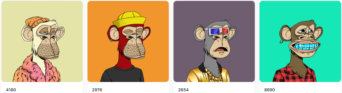
One category among all the spectrum of NFTs categories that has gained
remarkable prominence is the picture-for-profile. PFPs represent digital avatars
or profile images that users can adopt across various online platforms and social
media networks. BAYC, one PFP collection, is held by a few notable NBA
stars, singers and television hosts. Azuki’s NFT profile pics sold out in three
minutes and Okay Bears sold out all 10,000 NFTs in a day, bringing in a daily
record of $18 million in sales volume.

Focusing on this narrative, this research paper aims to contribute to the current knowledge landscape by conducting a thorough investigation into the
intricate determinants influencing the pricing of NFTs, with a specific focus on
the picture-for-profile category. Through an in-depth analysis of five distinct
NFT collections falling under this category, we seek to uncover the underly-
ing internal and external factors that propel market dynamics and ultimately
determine the intrinsic value of these digital assets.
In the subsequent sections of this research paper, we present the literature
review, providing an overview of the current knowledge of NFTs, yet still limited,
the methodology we used in this paper, as well as the database that we built,
the results for our 5 analyzed PFP collections, the discussion of these results
and the conclusion.
Literature Review
This literature review aims to explore the methodologies and findings of
several studies that shed light on the multifaceted realm of NFTs. By delving
into these different aspects, we aim to provide a comprehensive understanding
of the NFT ecosystem, its complexities, and its potential implications.
NFTs, or non-fungible tokens, represent tradable rights that can be securely
recorded as ownership tokens on the blockchain through the use of smart con-
tracts (Ko et al. 2022). While there are various definitions of NFTs, a simplified
explanation is that they are tokens that certify the uniqueness of digital assets
(Kapoor et al. 2022).
However, in order to gain a better understanding of these digital assets,
it is helpful to categorize them based on their different types. (Nadini et al.
2021) has identified six distinct groups of non-fungible tokens, namely Art,
Collectible, Games, Metaverse, Utility and Other. Although this categorization
provides a broad framework for discussing NFTs, the “Other” category is quite
vague and lacks precision. To notice this limitation, we can cite (Mazur, n.d.),
a research paper that delves into the risks and returns of NFTs and explores
various financial use cases, such as trading, liquidity mining, farming, collateral-
based loans, and fractional NFTs. These use cases, if classified, would all fall
under the broader classification of “Other”, not being very precise.
Upon comprehending the categorization of NFTs and their use cases, we
looked into the various factors that can influence the price of an NFT. In this
regard, (Kaczynski and Kominers 2021) examined the creation of NFT value
through several key aspects; the scarcity, which stems from the unique nature
of an NFT, making it highly desirable and valuable, the rarity, which is enhanced
when some creators intentionally limit the number of tokens they produce, the
authenticity, which involves the verification of an NFT’s uniqueness, the prove-
nance, which is related to the ownership history and transaction records of an
NFT, the popularity, which plays a important role when the collection is as-
sociated with renowned artists or celebrities, or when it has gained significant
attention on social media, and lastly, utility, which is an important factor to
analyze whether an NFT offers more practical use cases beyond being a mere picture.
Furthermore, the influence of visual features in the price of NFT is a well-
explored subject in the literature. For example, (Mekacher et al. 2022) thor-
oughly investigated the number of distinctive attributes linked to each NFT, as
well as the distribution of these attributes within the collection. Building upon
this idea, (Krasnoselskii, Madhwal, and Yanovich 2023) collected all attributes
from an NFT collection, measuring their rarity and proposing a rarity score. In
contrast, a different approach was taken by (Nadini et al. 2021) that considered
the overall image of each NFT instead of analyzing individual attributes sepa-
rately. Finally, (Alexander and Chen 2022) introduced the concept of grouping
NFTs with similar attributes, creating clusters and conducting separate analyses
for each cluster.
While these factors primarily encompass elements intrinsic to the NFT or
its collection, there are also external factors that may influence the NFT’s price.
For example, (Borri, Liu, and Tsyvinski 2022) investigated the influence of the
cryptocurrency market as well as traditional assets such as equity, commodities,
and currencies on NFT prices.
Finally, we looked into various economic models to modelize the price of
each NFT. When we have a number of observations on sales of objects that,
although individually unique, have some degree of commonality, and trades
are infrequent, all characteristics that we find in an NFT sale, we can apply
the Hedonic Regression (Galbraith and Hodgson 2018). The Hedonic method
was first proposed by (Court 1939) and then largely used and improved in the
literature, with a focus on the Real Estate and Art market. (Agnello, n.d.)
estimated the returns as well as the effects of various features of the paintings,
like their size, who is the author, where it was auctioned, the medium of painting
(e.g. oil, acrylic on canvas, panel, board, Masonite. . . ) on price. (Meese and
Wallace 1991) estimated house price for some cities in the United States of
America, considering for the feature variable the number of bathrooms and
bedrooms, finished square footage, total number of rooms, dwelling age, and for
the dummy variable the presence or absence of pools, fireplaces, assumability of
mortgage, mortgage type and zoning type.
Besides, this model incorporates external factors and features that can af-
fect house price, such as the impact of crime risk of property values (Linden
and Rockoff 2008), the relationship between the undergrounding electricity and
telecommunication network with house prices (McNair and Abelson 2010), and
the impact of Noosa national park on surrounding property values (Pearson,
Tisdell, and Lisle 2002).
However, it is important to note that it is not possible to include all potential
characteristics that may influence the price of an asset. (Epple 1987) highlighted
the issue of omitted variable bias, which poses a significant problem in hedonic
regression models. To mitigate this problem, one approach is to adapt the
hedonic model, which typically analyzes the price of a single asset, and instead
consider a pair of sales. The repeat sales model, proposed and improved by (Case
and Shiller 1987), is a powerful model that can estimate the house price index
without explicitly considering the attributes of the house. An adapted version of the Case and Shiller index is currently utilized by the S&P 500 to calculate
the house price index. While there is limited literature linking this method to
the NFT market, (Borri, Liu, and Tsyvinski 2022) employs the repeat sales
method to construct an overall index for the NFT market.
In parallel to the economic models, the emergence of machine learning and
artificial intelligence has provided opportunities to develop ML models for pre-
dicting NFT prices. (Nadini et al. 2021) employed a deep convolutional neural
network to extract the image feature and analyze their influence. Similarly,
(Mekacher et al. 2022) used the same approach to identify latent variables that
potentially drive the relationship between rarity and price. Moreover, (Jain,
Bruckmann, and McDougall, n.d.) built a recurrent neural network to uncover
the underlying factors affecting NFT prices, while (Alexander and Chen 2022)
applied ML techniques, such as random forest algorithm, to predict the NFT
rarity based on their attributes.
With that in mind, we can construct mathematical models to estimate the
price of NFTs and find the factors that influence its valuation, but it is also
important to consider alternative perspectives. According to (Kapoor et al.
2022), directly modeling NFT valuation as a mathematical economic system
may not be the most accurate approach. Instead, it should be viewed as a so-
cial phenomenon involving marketing schemes, the recognition and popularity
of the NFT. The role of social media has a significant impact on that valu-
ation and it emerges as a crucial factor of the NFT price. This perspective
aligns with previous research that has examined the impact of Twitter on stock
market prediction (Bollen, Mao, and Zeng 2011), highlighting the relevance of
social media in financial contexts. Additionally, this same article references the
Efficient Market Hypothesis, which suggests that stock markets are primarily
influenced by new information, such as news, rather than relying solely on past
and present prices. These insights encourage a holistic approach that incor-
porates social factors, market sentiment, and the timely incorporation of new
information alongside mathematical modelling when analysing NFT valuations.
Empirical Methodology
Before delving into the mathematical model, we believed that it was es-
sential to establish our own categorization framework to gain a comprehensive
understanding of the NFT landscape, as it follows:
1) Social / Membership: NFTs that can grant access to exclusive events and
communities.
2) Metaverse: NFTs that can represent plots of land on which it is possible to
construct buildings or organize events. This digital space enables activities such
as hosting online exhibitions or facilitating massive multiplayer video games.
3) Gaming: NFTs that are associated with any digital item from the domain
of online games. It can be in-game items, characters, skins, maps, tickets, etc.
4) Proof of ownership of a specific physical or digital item: NFTs that have
a physical artwork related in real life.
5) Financial NFTs: NFTs that represent fractional ownership of physical
assets (real estate, cars. . . ), stocks and bonds, futures and options contracts,
virtual currency-backed NFTs.
6) Music: NFTs that represent albums or music releases.
7) Domain name: NFTs that can simplify decentralized domains, such as
wallet addresses.
8) Pictures for profiles (PFPs): NFTs that were created to be displayed on
social media profiles.
9) Collectibles: NFTs that have been created to be used and are attached
to a project.
10) Photography: NFTs that represent unique photographs, often taken and
edited digitally.
11) Comics: NFTs that represent unique comic book pages, often featuring
digital art and storytelling
12) 3D Sculptures: NFTs that represent unique 3D sculptures, created using
3D modeling software and often animated or interactive.
13) Digital Paintings: NFTs that represent unique digital paintings, created
using digital tools and softwares.
14) Artistic Videos: NFTs that represent unique video works of art, often
including animation, motion graphics, and sound.
15) Mixed Media Art: NFTs that represent unique digital pieces that com-
bine multiple types of media, such as painting, sculpture, photography, and
digital design.
With the aid of this categorization framework, we can develop a comprehen-
sive overview of the NFT ecosystem, facilitating analysis of the potential factors
that may impact its pricing. We have classified these factors into two distinct
categories: internal and external.
Internal Factors:
1) Artist Popularity/Brand Recognition: This variable refers to the fame
and recognition of the artist or creator behind the NFT. The more popular or
well-known the creator, the more valuable the NFT may be.
2) Quality of Artwork/Visual Features: This variable refers to the aesthetic
value of the artwork or visual features of the NFT. The higher the quality and
appeal of the artwork or visual features, the more valuable the NFT may be.
This can also be seen as the value or appeal of the artwork from a market
perspective.
3) Number of NFTs (Scarcity): This variable refers to the number of NFTs
available in circulation. The scarcer the NFT collection is, the more valuable it
may be.
4) Rarity: This variable is similar to the previous one and refers to how
unique the characteristics in the NFT are. The more unique the attributes in
an NFT, the more valuable it may be.
5) Blockchain Technology: This variable refers to the blockchain chosen for
creating and maintaining the NFT. The more popular and widely used the
chosen blockchain, the more valuable the resulting NFT may become.
6) Added Utility: This variable refers to any additional benefits or uses that
the NFT may have beyond its intrinsic value. For example, if the NFT grants
access to exclusive content or events, it may be more valuable.
7) Historical Significance (OG NFTs): This variable refers to the historical
significance of the NFT, especially if it was one of the first NFTs ever created.
The more historical significance the NFT has, the more valuable it may be.
8) Process: This variable refers to the process of creating a collection with
respect to the various methods used by the artist.
External Factors:
1) Social Media: This variable refers to the impact that social media may
have on the value of the NFT. If the NFT is popular on social media platforms,
it may be more valuable.
2) Market Trends/Demand: This variable refers to the current market trends
and demand for NFTs. If there is a high demand for NFTs, the value of the
NFT may increase.
3) Economic Conditions: This variable refers to the overall economic con-
ditions, such as inflation, that may affect the value of the NFT. For example,
during an economic downturn, the value of NFTs may decrease.
By incorporating both internal and external factors, we aim to gain an ex-
tensive understanding of the various elements that can shape the value and de-
sirability of NFTs within the studied collections. We gathered the data focusing
on the most prominent PFP collections in terms of volume, namely CryptoP-
unk , Bored Ape Yacht Club, Mutant Ape Yacht Club, Azuki, CloneX, and
Moonbirds. We opted to exclude CryptoPunk from our analysis because it was
one of the first NFT collections launched in 2017, before the implementation
of the ERC-721 token protocol that is used nowadays. Consequently, relevant
historical sales data for that collection was not found, leading to its omission
from our research.
Initially, we turned to Etherscan, an Ethereum block explorer and analyt-
ics platform, to obtain the data, since all the collections mentioned are on the
Ethereum blockchain. While etherscan provided information on sales and mint-
ing, and we got the mint data for our analysis, we encountered an issue when
sales were conducted in currencies other than ETH, not being accurately repre-
sented. Furthermore, the traits data for each NFT was not available on Ether-
scan, leading us to search for another option.
Our next approach involved exploring Alchemy, a web3 developer platform,
to find the desired data. Unfortunately, we were unable to retrieve the traits
data for the collections, prompting us to quickly dismiss this option. Conse-
quently, we continued our search for a reliable source of NFT data.
Although Reservoir had the historical sales data, we could not rely on that
third option due to the presence of missing data when manually verifying the
information.
Ultimately, we turned to NFTPort, where we successfully obtained all the
desired data except for the mint price and mint date, which we got on Ether-
scan. For each collection, we retrieved the traits of all the NFTs, the historical sales data for each token ID, as well as the buyer and seller addresses. Ad-
ditionally, we obtained the sale prices in both ETH and USD, although, in
some instances, only the ETH price was available. To address this, we uti-
lized the historical price of that token to calculate the USD price, available at
www.coingecko.com/en/coins/ethereum.
We made a slight adjustment to the historical sales data to suit our model’s
requirements. Specifically, we observed that some NFTs were sold multiple times
on the same day with price differences of less than 5%. Such cases indicated that
these sales were driven purely by speculative motives. To streamline our dataset
and eliminate potential noise from speculative transactions, we decided to retain
only the first sale of each NFT on a given day, excluding any subsequent sales.
In addition to the NFT data, we also gathered various time series for further
analysis, such as the S&P 500 index from Yahoo Finance, the Federal Funds Rate
available at https://www.newyorkfed.org/markets/reference-rates/effr, and the
ETH price data from CoinGecko.
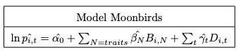
As mentioned in the literature review, we modeled our problem as a hedonic
model (Court 1939):

Before proceeding with the model, we first addressed the problem of mul-
ticollinearity, which occurs when two or more independent variables are highly
correlated, making it challenging to isolate their individual effects on the de-
pendent variable. To tackle this problem, we calculated the correlation matrix
for all independent variables in the dataset. This matrix reveals the pairwise
correlation between each pair of independent variables, ranging from -1 to +1,
where -1 indicates a perfect negative correlation, +1 represents a perfect positive
correlation, and 0 suggests no correlation.
Next, we established a threshold of ±0.7 for the correlation coefficient, and
if the correlation between two variables exceeded this threshold, we excluded one of them from the model. By doing so, we retained the most relevant and
informative predictors while mitigating the impact of multicollinearity.
To determine the coefficients of the Hedonic model, we adopted the Ordinary
Least Squares method (OLS), which minimizes the sum of the squared differ-
ences (residuals) between the observed dependent variable and the predicted
values generated by the linear equation.
It is worth noting that our NFT’s characteristics remain constant over time,
and thus our vector of features, denoted Bi,N , is the same for each period.
Greenlees (1982), Mark and Goldberg (1984) analyzed this special case when
the feature vector varies over the time, but we don’t need to treat our problem
in this way.
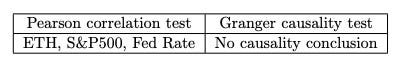
Following the coefficient estimation, we examined the correlation and causal-
ity between the regression coefficient related with the time, denoted as γt, and
three other time series: S&P 500 index, FED rate and ETH price.
To measure the correlation between two series, we utilized the Pearson Test,
which is a statistical test to assess the strength and direction of two variables, by
calculating the Pearson correlation coefficient (r). This coefficient ranges from -
1 to +1, where -1 represents a perfect negative linear relationship, +1 represents
a perfect positive linear relationship, and 0 indicates no linear relationship.
For measuring causality between two series, we employed the Granger Test,
which is a statistical test that helps to determine whether one time series can
predict another time series, revealing the temporal relationship between vari-
ables and assessing the predictive power of past values from one variable on
another one.
Results
Bored Ape Yacht Club
Proceeding with the methodology described in the previous section, we
started by analyzing the correlation between all the traits. For the Bored Ape
Yacht Club, we didn’t find any correlated traits (with the correlation matrix
coefficient higher than 0.7).
Following the steps, we ran our Hedonic Model to find the appropriate model to predict the collection price, considering only the statistically significant coeffi-
cients. We found that all coefficients were statistically significant at a significant
level of 0.05, but the coefficients related to the background feature.

We continued the analysis by measuring the linear relationship between the
estimated coefficients and its rarity and finally we ran a Pearson test and a
Granger test to verify the correlation and causality of the temporal estimated
coefficient and three other temporal series.


Mutant Ape Yacht Club
This collection is a particular one because it has a different type of mint for
some specific token ids: the last 20000 NFTs can only be minted if you have a
BAYC NFT (a detailed explanation will be given in the next section). Our first
approach was to treat all 30000 NFTs as equal.
We didn’t find any statistically significant coefficient.

As a second approach, we divided the collection into two: the first being
the 10000 NFTs (Token ID 0 to 9999) and the next 20000 (token id 10000 to
29999). The explanation of that division will be given in the next section.
For the first group, we found only 8 significant coefficients and we didn’t
continue the analysis for this first batch.
For the second group, we found the following model, with 764 statistically
significant coefficients, but with 260 not statistically significant coefficients.

Because of the high number of statistically insignificant coefficients, we de-
cided to not proceed the analysis for the second sample either.
Azuki
For the Azuki collection, we found 14 pairs with the correlation matrix co-
efficient higher than 0.7 and thus we excluded one of each pair from our feature
vector.


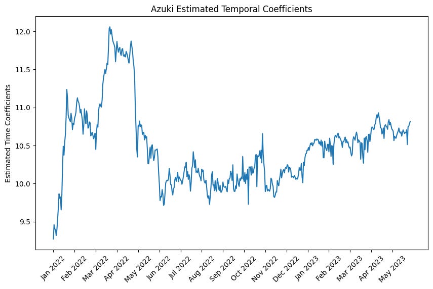
For the Hedonic Model, at a significant level of 0.05, we found that only the
temporal coefficients are significant to predict the price.

Following with the Pearson test and Granger test, we found that the esti-
mated temporal coefficients are correlated with the ETH price, S&P500 and
with the Fed Rate, and we found a causality with the S&P500 index with lag
2, 3, 4, and 5.
Since we didn’t have significant coefficients for the features, we didn’t verify
the relationship between them and rarity.

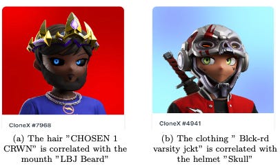
CloneX
For the CloneX collection, we found 8 correlated pairs of features and we
excluded one feature of each pair from our feature vector.
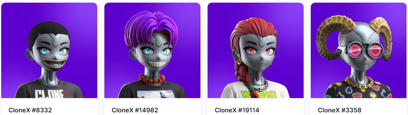
For this collection, we didn’t have a sufficient number of statistically signif-
icant coefficients. Only for these cases of features (Table 6).
Since we didn’t have enough coefficients, we didn’t proceed with the Granger
test, nor the Pearson test.

Moonbirds
For the Moonbirds collection, we found 16 correlated pairs of features and
we excluded one feature of each pair from our feature vector.


For the model, at a significance level of 0.05 we didn’t have any statistically
significant coefficients, but at 0.10 we found the following model:
Some traits were not statistically significant (Table 8).
We continued the analysis by measuring the linear relationship between the
estimated coefficients and its rarity and finally we ran a Pearson test and a
Granger test to verify the correlation and causality of the temporal estimated
coefficient and three other temporal series.


Apart from the individual analyses of each collection, we also conducted a
comparative assessment to derive general insights. The results are presented in
the following six charts:
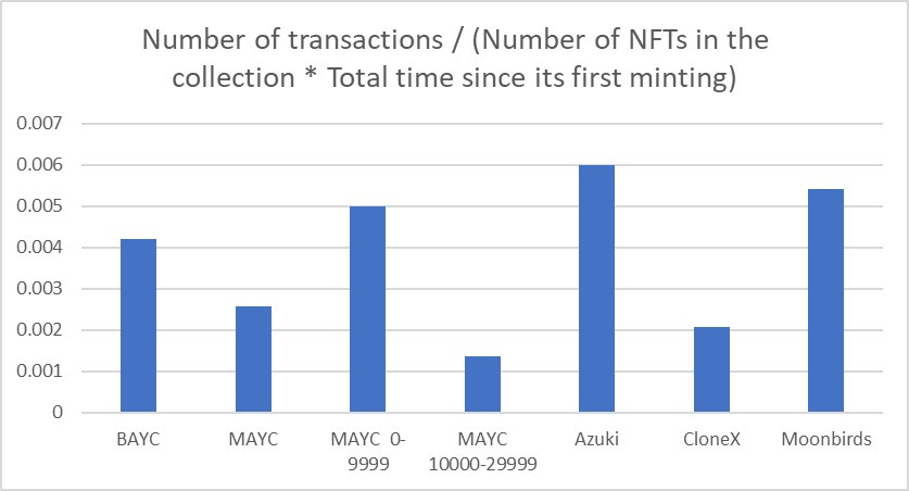
The first Chart represents the Number of transactions / (number of NFTs in
the collection * days since its first minting). This is a good KPI that we proposed
to analyze the frequency of transactions in a collection. It is important to notice
that if we decided to look only for the number of transactions, the number
would not be very meaningful: older and bigger collections tend to have more
transactions than newer and smaller ones. Then, with this KPI we can eliminate
these factors and normalize the number of transactions.
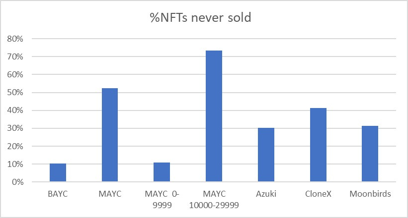
The second chart displays the percentage of NFTs in a collection that were
never sold.
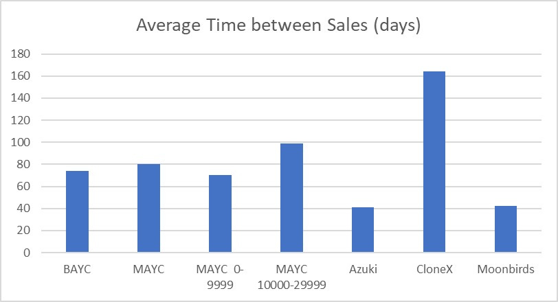
In the third chart, we observe the average time in days between sales of the
same NFT, including the time of the first sale.
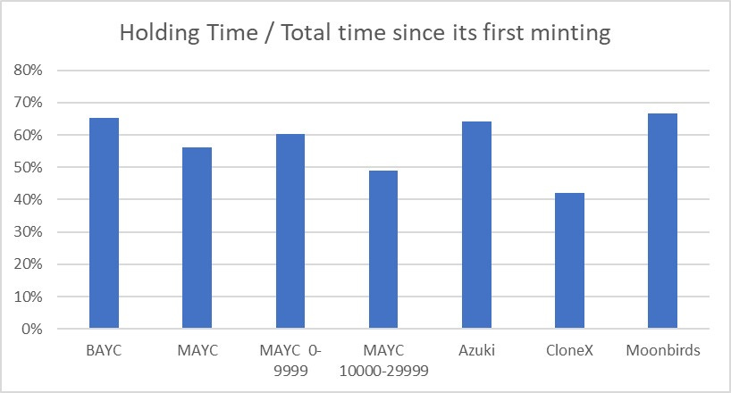
Chart four provides insights into how long people tend to keep their NFT
in their wallet. Again in this case, we proposed this KPI which we divide by
the total time since its first minting. The reason behind is that older collections
tend to have higher holding time than newer ones, because of its age.
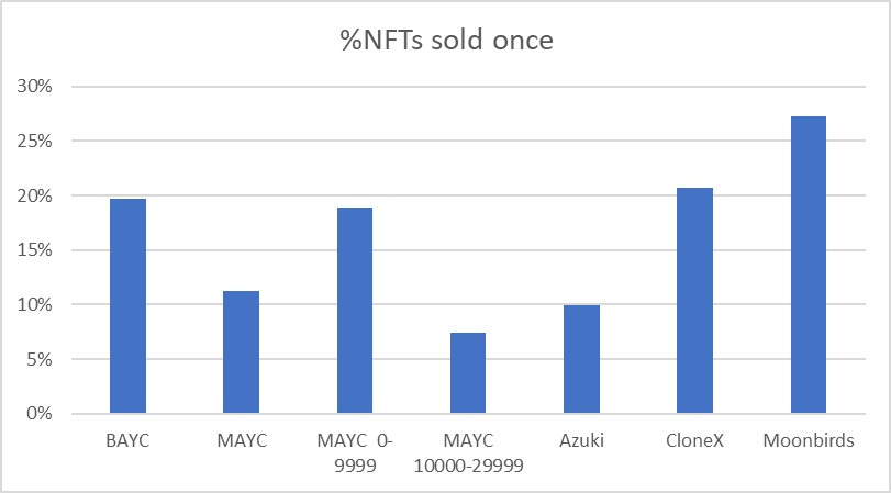
The fifth chart shows the percentage of NFTs that were sold only once.
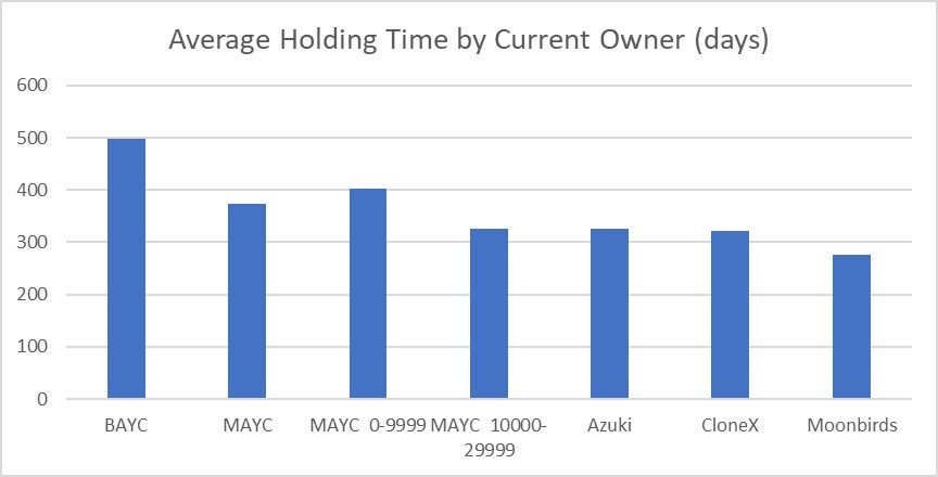
Lastly, the sixth chart highlights the holding time, which is the average time
that the actual owner of the NFT holds it.
Discussion
The findings from the analysis of the 5 PFP collections have yielded signif-
icant insights regarding our research question. They shed light on the charac-
teristics of these collections and the factors that may impact them. Notably,
for two collections (BAYC and Moonbirds), traits and aesthetics emerged as in-
fluential factors, suggesting that potential buyers consider the visual appeal of
the PFPs before making a purchase decision. On the other hand, for three col-
lections (BAYC, Azuki, and Moonbirds), external factors played a substantial
role in investors’ decision-making process. Lastly, the results for two collections
(CloneX and MAYC) were inconclusive, warranting further investigation.
Bored Ape Yacht Club and Moonbirds
Starting with Bored Ape Yacht Club (BAYC) and Moonbirds, the results
indicate that the feature vector of estimated coefficients plays a significant role
in influencing the price of NFTs, suggesting that potential buyers prioritize the
features and aesthetics of an NFT before making a purchase.
Moreover, when considering the percentage of total time that these two col-
lections were held (Figure 25), they stood out among the others. This reinforces
the idea that people value these NFTs and tend to hold them for more extended
periods because of personal preferences rather than speculative motives. No-
tably, the data showed that Moonbirds is the collection with the highest per-
centage of NFTs sold only once (Figure 26), exceeding 25%. On the other hand, BAYC is the collection where people hold onto their NFTs for the longest pe-
riod of time (Figure 27). These results provide further support to the notion
that individuals perceive NFTs from these collections as personal items of value
rather than mere speculative assets.
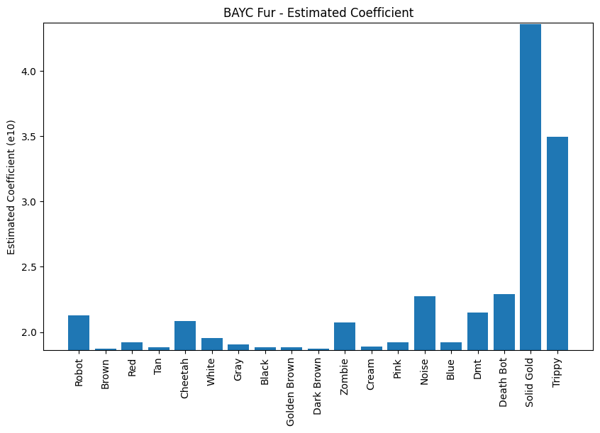
Looking deeper into the traits effects, we selected one trait from each collec-
tion to analyze its rarity influence. For the Bored Ape Yacht Club collection, we
focused on the “FUR” trait. In figure 5, our findings revealed that the “Solid
Gold Fur” is the rarest feature, accounting for less than 2% of the total NFTs
in the collection. Additionally, when exploring the average sale price of NFTs
in a determined type of fur (Figure 7), the Solid Gold Fur emerged as the most
expensive by a significant margin.
We attempted then to establish a linear relationship between rarity and price
(Figure 8), but the results were not highly conclusive (R2 = 0.16). That result
was led by some cases like the “Blue Fur”, which exhibited an average frequency
within the sample, and surprisingly possessed the lowest average price. This
complexity in the relationship between rarity and price hindered a strong linear
approximation.
Interestingly, all the estimated coefficients from our analysis were positive,
indicating that the presence of any trait, regardless of which one, would pos-
itively impact the predicted price of the NFT. This suggests that having a
particular trait, irrespective of its rarity, contributes to higher price predictions
for the NFT.
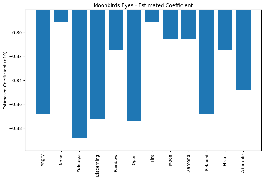
For the Moonbirds collection, we focused on the “eyes” trait to analyze
the relationship between rarity and price. Again in this case, we observed a
visual relationship between rarity and price, specifically, the “rainbow”, “fire”,
“moon”, “diamond”, and “heart” eyes were the scarcest within the collection
(Figure 18) and consequently, we found that NFTs featuring these unique eyes
traits, along with the “none” category, commanded the highest prices (Figure
20). However, trying to find a linear relationship to elucidate that relationship
was not very explanatory (Figure 21 shows R2 = 0.26).
Intriguingly, the behavior of the estimated coefficients differed from what we
found for the BAYC collection. For Moonbirds eyes, eyewear, headwear, and
outerwear, the coefficients were negative, indicating a downward pressure on the
predicted price. Conversely, the beak coefficients were all positives, suggesting
a positive influence on the price prediction. The coefficients for background,
body, and feathers were a mix of positive and negative values. For example,
legendary guardian, legendary emperor, legendary professor, legendary crescent,
legendary brave, and legendary sage feathers had positive coefficients, indicating
a preference for these unique features. On the other hand, feathers in colors like
gray, blue, white, purple, black, red, brown, prink, green, and none showed
negative coefficients, implying a lesser price impact, possibly due to their more
common occurrence.
Overall, that interaction between price and traits in the Moonbirds collec-
tions was very intriguing, as we exemplified with the eyes coefficients that were
all negatives, including the “none”, meaning that with or without this trait,
the price would decrease. This finding wasn’t entirely clear in our analysis and warrants further investigation to fully grasp the underlying factors involved in
it.
In our model, we not only identified the statistical significance of the feature
coefficients, but we also found that the temporal coefficients were significant.
After subjecting these coefficients to the Pearson correlation test, we observed
a strong correlation relationship between them and the three series we chose
to analyze: the ETH price, the S&P 500 index, and the Fed Rate. With the
ETH price, it is possible to see that the behavior of BAYC and Moonbids tem-
poral coefficients are similar to the ETH price behavior during certain “crypto
crashes” like the Luna crash in May 2022 and the FTX crash in November 2022.
However, it is essential to emphasize that correlation does not imply causation,
and we cannot establish a direct causal link based on these correlations.
Furthermore, we found correlations with two additional macroeconomic vari-
ables: the S&P5500 and the Fed Rate. This indicates that movements beyond
the NFT environment exhibit similar behavior to that observed within these
collections. While the exact causal mechanisms remain uncertain, these corre-
lations highlight the interconnectedness between broader economic conditions
and NFT pricing.
During the Granger causality test, for the BAYC collection, the analysis
yielded no evidence of causality between the temporal coefficients and the time
series proposed, even when exploring different time lags. In contrast, for the
Moonbirds collection, the causality test indicated a significant causation between
the temporal coefficient and the ETH price, with a lag of 5 time periods (Table
9). This implies that fluctuations in the ETH price play a contributory role in
shaping price variations within the Moonbirds collection.
This result is in line with (Ante 2021), who used data between January 2018
and April 2021 to demonstrate the impact of cryptocurrency markets on the
NFT market, finding that NFT sales were influenced by Bitcoin and Ether price
shocks. Furthermore, (Dowling 2021b) reinforces this result, as his exploration
of the NFT market in early 2021 suggested that cryptocurrency pricing may
provide valuable insights into NFT pricing patterns.
However, it is important to approach these findings with a degree of cau-
tion. Causality in complex systems like the NFT market can be influenced by
numerous interrelated factors, and the precise mechanisms at play may require
further investigation.
Azuki
In our investigation of the Azuki collection, we made intriguing discoveries
regarding the significance of feature and temporal coefficients. Different from
the first two collections, the feature coefficients were not statistically significant,
indicating that within this collection, people seem to be less concerned about
specific NFT features and more focused on market conditions and various in-
ternal and external factors. This observation suggests that the Azuki collection
may lean towards being a speculative collection, where buyers are driven by
investment opportunities rather than individual NFT characteristics.
Supporting this notion, Figure 24 reveals that Azuki exhibits the lowest
average time between sales, 41 days, suggesting that individuals tend to buy and
sell Azuki NFTs quickly, treating them more like short-term investments rather
than holding them for extended periods. In addition to that, we proposed a new
KPI that also corroborates with that result (Figure 22): number of transactions
per number of nfts in the collection per day since its first minting. Azuki was
on top of the other collections in that chart, showing its high trade frequency.
As we did not observe any statistically significant feature coefficients, we
did not explore their relationship with the rarity of traits within the Azuki
collection. Instead, we proceeded with correlation and causality tests to delve
further into the dynamics at play.
During our analysis, we discovered correlations between the three series we
examined with the temporal coefficients in the Azuki collection. Additionally,
the Granger causality test revealed that the S&P500 at lag 2,3,4,or 5, exhibited
a significant correlation with the Azuki NFT price. These findings align with
our previous observations, suggesting that investors may closely monitor the
behavior of the S&P500 to inform their investment decisions concerning specific
Azuki NFTs. Consequently, movements in the S&P500 are likely to influence
the overall price of the Azuki collection.
This connection between a market indicator and the Azuki NFT price high-
lights the speculative nature of the collection, where external market factors
hold sway over the NFT pricing dynamics.
That result diverged from the findings by (Aharon and Demir 2021), who
investigated NFTs’ connectedness with other financial assets during COVID-
19, concluding that NFTs have an independence from common asset classes
(equities, bond, currencies, gold, and oil).
The observed divergence in findings may be attributed to the difference in
the time frames analyzed. Aharon and Demir studied the period from January
2018 to June 2021, while Azuki’s first mint occurred in 2022. As the NFT market
rapidly evolves, early stages might not reflect its current state and hence, the
NFT landscape at the beginning of the study might differ significantly from the
present scenario. Therefore, considering the time gap is crucial to account for
the dynamic nature of the NFT market.
CloneX
Our next examination was CloneX and it posed unique challenges different
from the other collections. Regrettably, we did not find any statistically signifi-
cant coefficients in our model. This suggests that the model we proposed might
not be the most suitable for this particular collection.
One notable aspect of CloneX is its status as the oldest collection among all
those we studied, with over two years since its first minting. However, surpris-
ingly, approximately 40% of CloneX NFTs remain unsold (Figure 23). This sig-
nificant number of unsold NFTs introduces complexities that impact the model’s
precision in capturing all influences, particularly concerning the features coef-
ficients. Since only 60% of the NFTs were sold at least once, the model only considers the features of those sold NFTs, leaving some traits that were never
sold unaccounted for. This limitation has a detrimental effect on the reliability
of the coefficients within the model.
Regarding temporal coefficients, we observed that CloneX exhibited the
highest value in the Average Time Between Sales, reaching 164 days (Figure
24) . This implies that CloneX NFTs are not traded frequently, making it chal-
lenging to incorporate the temporal aspect into the model due to the scarcity
of sales data.
Given these limitations and the lack of sufficient statistically significant co-
efficients, we made the decision to not pursue further tests of correlation and
causality. Instead, we acknowledge the uniqueness of the CloneX collection and
the difficulties it presents in analyzing its pricing dynamics.
Mutant Ape Yacht Club
MAYC stands out as another distinct collection that posed its own unique
challenges during our analysis. Running the model for all NFTs within the
collection (token ID from 0 to 29999), did not yield any statistically significant
coefficients. Similar to CloneX, MAYC’s peculiarities influenced these results.
One notable aspect of MAYC is that over 50% of its NFTs were never
sold (Figure 23), surpassing even the percentage observed in CloneX. Conse-
quently,certain traits within MAYC were never considered in our model, im-
pacting the precision of feature coefficients. This lack of sales data for a signif-
icant portion of the collection introduced complexities in the comprehension of
the price dynamics.
Furthermore, the average time between sales for Mutant Ape Yacht Club
NFTs is 80 days (Figure 24), outstanding the duration observed in BAYC,
Azuki, and Moonbirds collections. That infrequency of sales further complicated
the inclusion of temporal effects in the model, making it challenging to capture
the dynamics of pricing fluctuations.
Given these challenges, our initial analysis, a naive one, faced limitations
in fully grasping the pricing behavior within the MAYC collection. However,
acknowledging these unique characteristics motivates us to explore alternative
approaches and refine our methodology.
We made a deliberate division, creating two distinct sub-collections.The first
collection comprises token IDs ranging from 0 to 9999, while the second collec-
tion includes token IDs from10 to 29999. The division is not arbitrary; it aligns
with significant differences in the minting process and requirements for each
group.
The first 10000 MAYC NFTs were generated through the usual process of AI
image generator, where a random vector of features creates unique NFTs that
can be minted by anyone in the community. This approach is consistent with
the typical NFT minting process, making this subset a representative sample of
conventional NFTs within the MAYC collection.
The second group, however, follows a distinctive protocol for minting. To
acquire a Mutant Ape Yacht Club NFT from this subset, individuals need to possess a Bored Ape Yacht Club NFT, and additionally, they require a special
element called “Serum”, available in two types: number 1 and number 2. With
these prerequisites met, individuals can mint their MAYC NFT, whose process
will follow the same steps as the first group, through an AI image generator.
This strategic division enabled us to examine two distinct categories within
the MAYC collection, shedding light on the contrasting dynamics between con-
ventional minting and the exclusive requirements for minting within the second
group.
During our analysis of the first part of the MAYC collection (token IDs
0-9999), we encountered an unexpected result. Despite a high percentage of
NFTs sold, Figure 23 shows only 11% of NFTs in that group remained unsold,
a considerable number of transactions per NFT per time of existence (Figure
22), and a low average time between sales (Figure 24), we did not find any
statistically significant coefficient.
These characteristics led us to expect a similar behavior to that of BAYC and
Moonbirds collections, where the feature and temporal coefficients significantly
influenced price predictions. However, as we have seen, this was not the case.
At this point, we have not yet determined the reasons behind this outcome, and
further investigation is needed to understand the implications fully.
On the other hand, the second part of MAYC collection (token IDs 10000-
29999) exhibited a behavior more akin to the BAYC and Moonbirds collections.
These NFTs stand out as unique with its way of minting, fostering a sense of
pertinence among collectors that mint it. As a result, a significant portion of
these MAYC NFTs were never sold (over 70% according to Figure 23).
In addition to that, Figure 22 reveals infrequent trading activity for these
NFTs, suggesting that collectors tend to hold onto their NFTs and this sub-
collection has the second-highest average time between sales (Figure 24), behind
CloneX. This aspect emphasizes the collector-oriented nature of the owners of
these NFTs. Despite all these characteristics, we still observed some temporal
influence in the predicted price (there were some significant temporal coefficients
in our model), indicating that those who decide to sell their minted NFTs may
consider market conditions in their decision-making.
Due to the absence of a continuous time series for our temporal coefficients,
with some coefficients turning out to be statistically insignificant, we made the
decision to not proceed with the correlation and causality tests. Similarly, we
encountered some features coefficients that lacked significance, resulting in miss-
ing coefficients. As a consequence, we opted against verifying the relationship
between the rarity of traits and their estimated coefficients.
The limitations posed by these missing coefficients in both temporal and fea-
ture coefficients prevented us from conducting further analyses to explore corre-
lations and causal relationships. Recognizing these constraints, we acknowledge
the need for a more comprehensive dataset to gain deeper insights into the
dynamics and influences governing the NFT pricing within the collection.
In conclusion, the results emphasized that the aesthetics and features of
NFTs have a significant impact on the pricing of BAYC and moonbirds, and
people tend to hold NFTs they appreciate for more extended periods. The Moonbirds collection, despite having fewer transactions overall, witnessed a sub-
stantial percentage of NFTs sold only once, showcasing the initial intention of
buyers to retain these items in their wallets. The Azuki collection appeared as
a speculative collection, with external market factors influencing its pricing dy-
namics more than specific NFT features. CloneX and MAYC presented unique
challenges in analyzing their pricing behavior due to their particularities and
their data availability.
Conclusion
In this research, we conducted a comprehensive analysis of five PFP collec-
tions, identifying the factors influencing the pricing dynamics of these digital
assets. Through rigorous examination, we made significant findings that con-
tributed to our understanding of the NFT market.
Firstly, we discovered that certain collections possess a speculative factor,
wherein the NFT prices are influenced by external market conditions. For
instance, the Azuki collection demonstrated a strong correlation between its
NFT prices and the S&P 500 index, indicating a close relationship between
the broader economy and the pricing dynamics of these NFTs. On the other
hand, Moonbirds exhibited a causal relationship with fluctuations in the ETH
price, suggesting that market movements in the Ethereum cryptocurrency play
a contributory role in shaping price variations within the collection.
Secondly, we observed that some collections had an appeal factor, where
NFT prices were influenced by intrinsic factors such as aesthetics features. No-
tably, Bored Ape Yacht Club and Moonbirds collections showed correlation
between specific NFT features and their prices, indicating that potential buyers
prioritize visual appeal and unique traits before making a purchase decision.
In all cases where a temporal effect was significant in the model, the ETH
price, S&P500, and Fed Rate exhibited correlations with the temporal coeffi-
cients estimated.
However, while our research yielded valuable insights for some collections,
we also encountered challenges in constructing a precise model for the Mutant
Ape Yacht Club and CloneX collections. The complexity and uniqueness of
these collections hindered a robust analysis. As a result, further investigation
is required to provide explanations for the difficulties encountered and to gain
deeper insights into the dynamics driving the pricing behavior within these
collections.
Moving forward, future research could apply the repeat sales method to the
Azuki collection, given its speculative nature, and also for MAYC and CloneX,
trying to identify the underlying pricing patterns and relationships.
In addition to traditional econometric approaches, future research papers
could employ machine learning models to analyze NFT pricing dynamics. Lever-
aging machine learning algorithms could help identify complex patterns and rela-
tionships between NFT characteristics, external factors, and transaction prices.
Another approach for exploration is the influence of social media platforms on NFT pricing and price volatility. Treating NFT price volatility as a social
phenomenon rather than merely a mathematical or economic problem would
provide a more comprehensive understanding of NFT market behavior and the
role of social influence.
Lastly, expanding the research to explore other NFT categories beyond PFPs
is essential for gaining a holistic view of the NFT market. Each category may
possess distinct characteristics, driving factors, and market dynamics. Conduct-
ing similar analyses for other categories, such as virtual real estate, digital art,
and gaming NFTs, would enrich the overall understanding of the entire NFT
ecosystem. By broadening the scope of the study, we can capture the diver-
sity and complexities of NFT markets, contributing to a more comprehensive
knowledge base for the digital asset space.
References
Agnello, Richard J. n.d. “INVESTMENT RETURNS AND RISK FOR
ART:” EASTERN ECONOMIC JOURNAL.Aharon, David Y., and Ender Demir. 2021. ”NFTs and asset class spillovers:
Lessons from the period around the COVID-19 pandemic.” Finance Research
Letters 47: 102515.Alexander, Carol, and Xi Chen. 2022. “Rarity Metrics for Non-Fungible
Tokens.” SSRN Electronic Journal. https://doi.org/10.2139/ssrn.4242042.Ante, Lennart. 2021. ”The non-fungible token (NFT) market and its rela-
tionship with Bitcoin and Ethereum.” FinTech 1, no. 3: 216-224.Borri, Nicola, Yukun Liu, and Aleh Tsyvinski. 2022. “The Economics of
Non-Fungible Tokens.” SSRN Electronic Journal. https://doi.org/10.2139/ssrn.
4052045.Case, Karl, and Robert Shiller. 1987. “Prices of Single Family Homes Since
1970: New Indexes for Four Cities.” w2393. Cambridge, MA: National Bureau
of Economic Research. https://doi.org/10.3386/w2393.Court, Andrew. 1939. “Hedonic price indexes with automotive examples”,
in “The Dynamics of Automobile Demand”, General Motors, New York, pp.
98.Dowling, Michael. 2021. ”Is non-fungible token pricing driven by cryptocur-
rencies?.” Finance Research Letters 44: 102097.Epple, D. 1987. Hedonic prices and implicit markets: Estimating demand
and supply functions for differentiated products. Journal of Political Economy,
95(1), 59–80.Galbraith, John, and Douglas Hodgson. 2018. “Econometric Fine Art Val-
uation by Combining Hedonic and Repeat-Sales Information.” Econometrics 6
(3): 32. https://doi.org/10.3390/econometrics6030032.Greenlees, J. S. 1982. An Empirical Evaluation of the CPI Home Purchase
Index, 1973-1978, Journal of the American Real Estate and Urban Economics
Association, 10:1, 1-24.Jain, Shrey, Camille Bruckmann, and Chase McDougall. n.d. “NFT Ap-
praisal Prediction: Utilizing Search Trends, Public Market Data, Linear Re-
gression and Recurrent Neural Networks.”Kapoor, Arnav, Dipanwita Guhathakurta, Mehul Mathur, Rupanshu Yadav,
Manish Gupta, and Ponnurangam Kumaraguru. 2022. “TweetBoost: Influence
of Social Media on NFT Valuation.” arXiv. http://arxiv.org/abs/2201.08373.Kaczynski, Steve, and Scott Duke Kominers. 2021. “How NFTs Create
Value.” Harvard Business Review. November 10, 2021. https://hbr.org/2021/
11/how-nfts-create-value.Kireyev, Pavel, and Ruiqi Lin. n.d. “Infinite but Rare: Valuation and
Pricing in Marketplaces for Blockchain-Based Nonfungible Tokens.”Ko, Hyungjin, Bumho Son, Yunyoung Lee, Huisu Jang, and Jaewook Lee.
2022. “The Economic Value of NFT: Evidence from a Portfolio Analysis Us-
ing Mean–Variance Framework.” Finance Research Letters 47 (June): 102784.
https://doi.org/10.1016/j.frl.2022.102784.Krasnoselskii, Mikhail, Yash Madhwal, and Yury Yanovich. 2023. “KRA-
MER: Interpretable Rarity Meter for Crypto Collectibles.” IEEE Access 11:
4283–90. https://doi.org/10.1109/ACCESS.2023.3236080.Linden, Leigh, and Jonah E Rockoff. 2008. “Estimates of the Impact of
Crime Risk on Property Values from Megan’s Laws.” American Economic Re-
view 98 (3): 1103–27. https://doi.org/10.1257/aer.98.3.1103.Mazur, Mieszko. n.d. “Non-Fungible Tokens (NFT). The Analysis of Risk
and Return.”Mark, J.H. and M.A. Goldberg, 1984, Alternative housing price indices: An
evaluation, AREUEA Journal 12, 3&49.McNair, Ben, and Peter Abelson. 2010. “Estimating the Value of Under-
grounding Electricity and Telecommunications Networks.” Australian Economic
Review 43 (4): 376–88. https://doi.org/10.1111/j.1467-8462.2010.00608.x.Meese, Richard, Wallace, Nancy, 1991. Nonparametric estimation of dy-
namic hedonic price models and the construction of residential housing price
indices. Real Estate Econ. 19 (3), 308–332. http://dx.doi.org/10.1111/1540-
6229.00555.Mekacher, Amin, Alberto Bracci, Matthieu Nadini, Mauro Martino, Laura
Alessandretti, Luca Maria Aiello, and Andrea Baronchelli. 2022. “Hetero-
geneous Rarity Patterns Drive Price Dynamics in NFT Collections.” arXiv.
http://arxiv.org/abs/2204.10243.Nadini, Matthieu, Laura Alessandretti, Flavio Di Giacinto, Mauro Martino,
Luca Maria Aiello, and Andrea Baronchelli. 2021. “Mapping the NFT Revolu-
tion: Market Trends, Trade Networks, and Visual Features.” Scientific Reports
11 (1): 20902. https://doi.org/10.1038/s41598-021-00053-8.Pearson, L.J., C. Tisdell, and A.T. Lisle. 2002. “The Impact of Noosa
National Park on Surrounding Property Values: An Application of the Hedonic
Price Method.” Economic Analysis and Policy 32 (2): 155–71. https://doi.org/
10.1016/S0313-5926(02)50023-0.Schnoering, Hugo, and Hugo Inzirillo. 2022. “Constructing a NFT Price
Index and Applications.” arXiv. http://arxiv.org/abs/2202.08966.Wen, Audrey Elizabeth, and HoiYat Wong. 2021. “Bidder and Seller
Strategies in Online Auctions: A Review:” In . Guangzhou, China. https:
//doi.org/10.2991/assehr.k.211209.325.